본 게시글의 원문은 Yann Debray의 MATLAB with Python Book 입니다. 해당 책은 MIT 라이센스를 따르기 때문에 개인적으로 번역하여 재배포 합니다. 본 포스팅에는 추후 유료 수익을 위한 광고가 부착될 수도 있습니다.
MIT License

Copyright (c) 2023 Yann Debray

Permission is hereby granted, free of charge, to any person obtaining a copy
of this software and associated documentation files (the "Software"), to deal
in the Software without restriction, including without limitation the rights
to use, copy, modify, merge, publish, distribute, sublicense, and/or sell
copies of the Software, and to permit persons to whom the Software is
furnished to do so, subject to the following conditions:

The above copyright notice and this permission notice shall be included in all
copies or substantial portions of the Software.

THE SOFTWARE IS PROVIDED "AS IS", WITHOUT WARRANTY OF ANY KIND, EXPRESS OR
IMPLIED, INCLUDING BUT NOT LIMITED TO THE WARRANTIES OF MERCHANTABILITY,
FITNESS FOR A PARTICULAR PURPOSE AND NONINFRINGEMENT. IN NO EVENT SHALL THE
AUTHORS OR COPYRIGHT HOLDERS BE LIABLE FOR ANY CLAIM, DAMAGES OR OTHER
LIABILITY, WHETHER IN AN ACTION OF CONTRACT, TORT OR OTHERWISE, ARISING FROM,
OUT OF OR IN CONNECTION WITH THE SOFTWARE OR THE USE OR OTHER DEALINGS IN THE
SOFTWARE.
본 게시물에서 활용된 소스 코드들은 모두 Yann Debray의 GitHub Repo에서 확인할 수 있습니다.
5.3. MATLAB에서 TensorFlow 모델 가져오기
TensorFlow 및 ONNX 모델 가져오기/내보내기 기능을 설명하기 위해 자율 주행 사용 사례 주변의 작업 흐름을 살펴보겠습니다.

데이터는 Udacity의 간단한 오픈 소스 주행 시뮬레이터에서 생성됩니다.
그리고 모델은 NVIDIA의 자율 주행을 위한 엔드-투-엔드 학습에 대한 실제 실험에서 가져왔습니다.

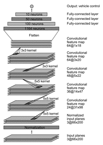
신경망의 입력은 카메라에서 온 이미지이고 출력은 조향 각도를 예측하는 것입니다(-1부터 1까지).
이 문제를 왼쪽에서 오른쪽으로 5개의 클래스로 단순화하겠습니다.
(선택 사항) CPU에서 훈련에 4개의 워커를 사용하기 위해 병렬 풀을 설정합니다.
p = gcp('nocreate'); % 풀이 없으면 새로 생성하지 않음.
if isempty(p)
   parpool()
else
    poolsize = p.NumWorkers
end
UDACITY 시뮬레이터에서 생성된 이미지 위치와 조향 각도의 참값이 포함된 CSV 파일을 가져옵니다.
filename = "driving_log.csv";
drivinglog = import_driving_log(filename);
drivinglog = drivinglog(2:end, :);
| VarName1 | center | left | right | steering | throttle | reverse | speed | |
|---|---|---|---|---|---|---|---|---|
| 1 | 0 | “center_2021_04_25_1… | “left_202104_25_11… | “right_2021_04_25_11… | 0 | 0 | 0 | 0 |
| 2 | 1 | “center_2021_04_25_1… | “left_202104_25_11… | “right_2021_04_25_11… | 0 | 0 | 0 | 0 |
| 3 | 2 | “center_2021_04_25_1… | “left_202104_25_11… | “right_2021_04_25_11… | 0 | 0 | 0 | 0 |
| 4 | 3 | “center_2021_04_25_1… | “left_202104_25_11… | “right_2021_04_25_11… | 0 | 0 | 0 | 0 |
| 5 | 4 | “center_2021_04_25_1… | “left_202104_25_11… | “right_2021_04_25_11… | 0 | 0 | 0 | 0 |
데이터 준비
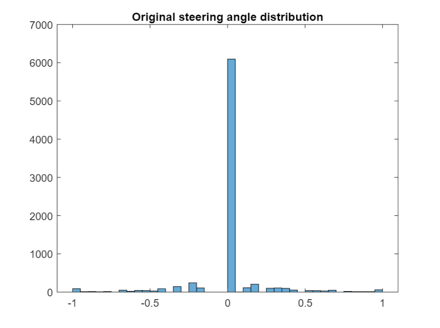
조향 각도의 범위를 분석하여 최적의 클래스 값을 찾습니다.
figure;
histogram(drivinglog.steering);
title("Original steering angle distribution");
discretize를 사용하여 조향 각도를 이산적인 구간으로 그룹화합니다.
steeringLimits = [-1 -0.5 -0.05 0 0.05 0.5 1];
steeringClasses = discretize(drivinglog.steering, steeringLimits, 'categorical');
classNames = categories(steeringClasses);
0도에 가까운 각도를 나타내는 두 개의 구간을 병합합니다.
steeringClasses = mergecats(steeringClasses,["[-0.05, 0)","[0, 0.05)"], "0.0");
histogramClasses = histogram(steeringClasses);
title("Angle distribution discretized (5 categories)");

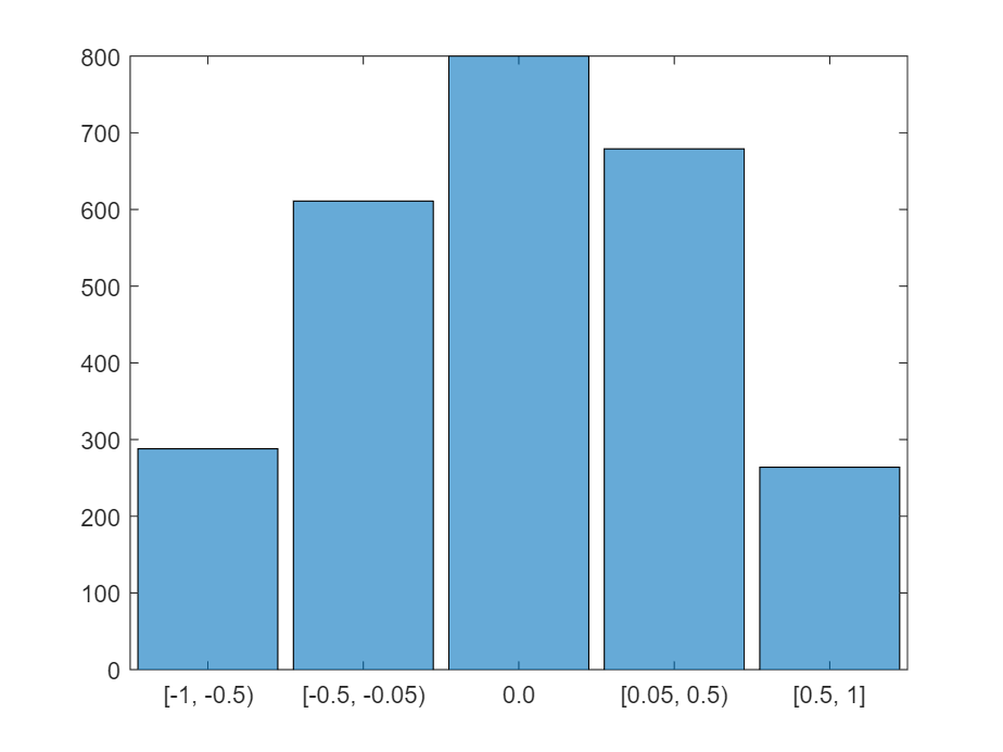
이미지 데이터 스토어 생성 및 데이터 균형 조정 (언더샘플링)
이전 히스토그램에서 데이터셋이 매우 불균형함을 보여줍니다. countEachLabel을 사용하여 각 클래스의 인스턴스 수를 확인합니다.
imds = imageDatastore("sim_data/"+drivinglog.center,"Labels", steeringClasses);
countEachLabel(imds)
| Label | Count | |
|---|---|---|
| 1 | [-1, -0.5) | 288 |
| 2 | [-0.5, -0.05) | 611 |
| 3 | 0 | 6093 |
| 4 | [0.05, 0.5) | 679 |
| 5 | [0.5,1] | 264 |
균형이 맞지 않은 클래스에서 유지할 샘플 수와 이러한 샘플을 무작위로 선택합니다.
maxSamples = 800;
countLabel = countEachLabel(imds);
[~, unbalancedLabelIdx] = max(countLabel.Count);
unbalanced = imds.Labels == countLabel.Label(unbalancedLabelIdx);
idx = find(unbalanced);
randomIdx = randperm(numel(idx));
downsampled = idx(randomIdx(1:maxSamples));
retained = [find(~unbalanced) ; downsampled];
imds = subset(imds, retained');
histogram(imds.Labels)
데이터셋을 학습, 검증 및 테스트로 분리
데이터 중 90%를 학습에, 나머지를 테스트 및 검증에 사용하기 위해 추출합니다.
[imdsTrain, imdsValid,imdsTest] = splitEachLabel(imds, 0.9, 0.05, 0.05);
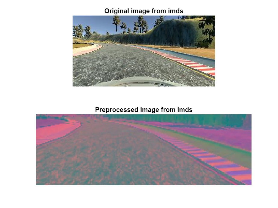
이미지 전처리
이미지를 크기 조정하고 YCbCr 색 공간으로 변환하여 전처리합니다.
trainData = transform(imdsTrain, @imagePreprocess, "IncludeInfo", true);
testData = transform(imdsTest, @imagePreprocess, "IncludeInfo", true);
valData = transform(imdsValid, @imagePreprocess, "IncludeInfo", true);
imds_origI = imdsTrain.read;
imds_newI = trainData.read{1};
subplot(211), imshow(imds_origI), title("imds의 원본 이미지")
subplot(212), imshow(imds_newI), title("imds의 전처리된 이미지")
모델 수정:
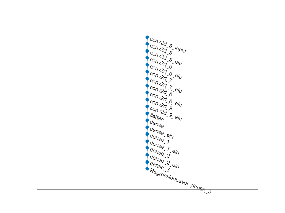
Keras 모델에서 네트워크를 로드하고 Deep Network Designer를 사용하여 표시합니다.
모델을 SavedModel 형식으로 저장하고 가져오는 것이 권장되며 (경고 메시지가 표시될 수 있음), HDF5 형식보다 더 우수한 결과를 얻을 수 있습니다.
layers = importKerasLayers("tf_model.h5")
layers =
  20x1 Layer array with layers:

     1   'conv2d_5_input'            Image Input         66x200x3 images
     2   'conv2d_5'                  2-D Convolution     24 5x5 convolutions with stride [2  2] and padding [0  0  0  0]
     3   'conv2d_5_elu'              ELU                 ELU with Alpha 1
     4   'conv2d_6'                  2-D Convolution     36 5x5 convolutions with stride [2  2] and padding [0  0  0  0]
     5   'conv2d_6_elu'              ELU                 ELU with Alpha 1
     6   'conv2d_7'                  2-D Convolution     48 5x5 convolutions with stride [2  2] and padding [0  0  0  0]
     7   'conv2d_7_elu'              ELU                 ELU with Alpha 1
     8   'conv2d_8'                  2-D Convolution     64 3x3 convolutions with stride [1  1] and padding [0  0  0  0]
     9   'conv2d_8_elu'              ELU                 ELU with Alpha 1
    10   'conv2d_9'                  2-D Convolution     64 3x3 convolutions with stride [1  1] and padding [0  0  0  0]
    11   'conv2d_9_elu'              ELU                 ELU with Alpha 1
    12   'flatten'                   Keras Flatten       Flatten activations into 1-D assuming C-style (row-major) order
    13   'dense'                     Fully Connected     100 fully connected layer
    14   'dense_elu'                 ELU                 ELU with Alpha 1
    15   'dense_1'                   Fully Connected     50 fully connected layer
    16   'dense_1_elu'               ELU                 ELU with Alpha 1
    17   'dense_2'                   Fully Connected     10 fully connected layer
    18   'dense_2_elu'               ELU                 ELU with Alpha 1
    19   'dense_3'                   Fully Connected     1 fully connected layer
    20   'RegressionLayer_dense_3'   Regression Output   mean-squared-error
deepNetworkDesigner(layers)
회귀에 사용된 마지막 레이어를 제거하고 5개 클래스로 분류하는 레이어를 추가합니다 (그런 다음 넷을 layers_1로 내보냄).

(프로그래밍 대체 방법) 회귀에 사용된 레이어를 제거하고 5개 클래스로 분류하는 레이어를 추가합니다.
netGraph = layerGraph(layers);
clf; plot(netGraph)
classificationLayers = [fullyConnectedLayer(5,"Name","dense_3"), ...
                        softmaxLayer("Name","softmax"), ...
                        classificationLayer("Name","classoutput")];
netGraph = removeLayers(netGraph, {'dense_3', 'RegressionLayer_dense_3'});
netGraph = addLayers(netGraph,classificationLayers);
layers_1 = netGraph.Layers
layers_1 =
  21x1 Layer array with layers:

     1   'conv2d_5_input'   Image Input             66x200x3 images
     2   'conv2d_5'         2-D Convolution         24 5x5 convolutions with stride [2  2] and padding [0  0  0  0]
     3   'conv2d_5_elu'     ELU                     ELU with Alpha 1
     4   'conv2d_6'         2-D Convolution         36 5x5 convolutions with stride [2  2] and padding [0  0  0  0]
     5   'conv2d_6_elu'     ELU                     ELU with Alpha 1
     6   'conv2d_7'         2-D Convolution         48 5x5 convolutions with stride [2  2] and padding [0  0  0  0]
     7   'conv2d_7_elu'     ELU                     ELU with Alpha 1
     8   'conv2d_8'         2-D Convolution         64 3x3 convolutions with stride [1  1] and padding [0  0  0  0]
     9   'conv2d_8_elu'     ELU                     ELU with Alpha 1
    10   'conv2d_9'         2-D Convolution         64 3x3 convolutions with stride [1  1] and padding [0  0  0  0]
    11   'conv2d_9_elu'     ELU                     ELU with Alpha 1
    12   'flatten'          Keras Flatten           Flatten activations into 1-D assuming C-style (row-major) order
    13   'dense'            Fully Connected         100 fully connected layer
    14   'dense_elu'        ELU                     ELU with Alpha 1
    15   'dense_1'          Fully Connected         50 fully connected layer
    16   'dense_1_elu'      ELU                     ELU with Alpha 1
    17   'dense_2'          Fully Connected         10 fully connected layer
    18   'dense_2_elu'      ELU                     ELU with Alpha 1
    19   'dense_3'          Fully Connected         5 fully connected layer
    20   'softmax'          Softmax                 softmax
    21   'classoutput'      Classification Output   crossentropyex
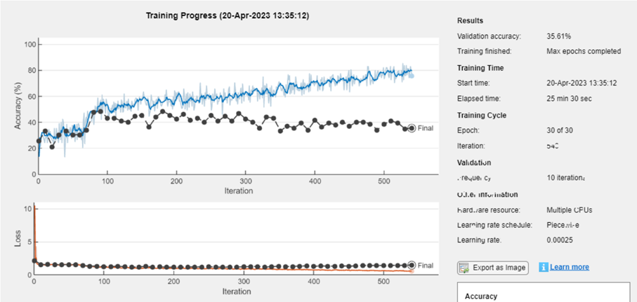
모델 훈련: (여기서는 CPU를 사용하지만, GPU에서 속도를 높이는 것을 권장합니다)
initialLearnRate = 0.001;
maxEpochs = 30;
miniBatchSize = 100;
options = trainingOptions("adam", ...
    "MaxEpochs",maxEpochs, ...
    "InitialLearnRate",initialLearnRate, ...
    "Plots","training-progress",  ...
    "ValidationData",valData, ...
    "ValidationFrequency",10, ...
    "LearnRateSchedule","piecewise", ...
    "LearnRateDropPeriod",10, ...
    "LearnRateDropFactor",0.5, ...
    "ExecutionEnvironment","parallel",...
    "Shuffle","every-epoch");
net = trainNetwork(trainData, layers_1, options);
모델 저장: 새로 훈련된 네트워크를 MAT 형식으로 저장합니다.
model_name = "net-class-30-1e-4-drop10-0_5"; % classification-epochs-learning_rate-drop_period-drop_factor
save(model_name + ".mat", "net")
ONNXNetwork 형식으로 내보냅니다.
exportONNXNetwork(net, model_name + ".onnx")
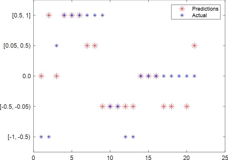
모델 테스트:
테스트 데이터셋을 사용하여 조향 각도의 예측 값과 실제 값의 그래프를 그립니다.
model_name = "net-class-30-1e-4-drop10-0_5"; % classification-epochs-learning_rate-drop_period-drop_factor
load(model_name+".mat","net")
predSteering = classify(net, testData);
figure
startTest = 80;
endTest = 100;
plot(predSteering(startTest:endTest), 'r*', "MarkerSize",10)
hold on
plot(imdsTest.Labels(startTest:endTest), 'b*')
legend("Predictions", "Actual")
hold off
혼동 행렬 표시:
혼동 행렬을 표시합니다.
confMat = confusionmat(imdsTest.Labels, predSteering);
confusionchart(confMat)
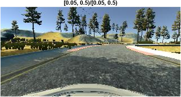
테스트 이미지와 예측된 라벨 표시:
테스트 이미지와 예측된 라벨, 그리고 실제 라벨을 표시합니다.
numberImages = length(imdsTest.Labels);
i = 42;
img = readimage(imdsTest, i);
imshow(img), title(char(imdsTest.Labels(i)) + "/" + char(predSteering(i)));
Helper Functions
function drivinglog = import_driving_log(filename, dataLines)
%IMPORTFILE Import data from a text file
%  DRIVINGLOG = IMPORTFILE(FILENAME) reads data from text file FILENAME
%  for the default selection.  Returns the data as a table.
%
%  DRIVINGLOG = IMPORTFILE(FILE, DATALINES) reads data for the specified
%  row interval(s) of text file FILENAME. Specify DATALINES as a
%  positive scalar integer or a N-by-2 array of positive scalar integers
%  for dis-contiguous row intervals.
%
%  See also READTABLE.
%
% Auto-generated by MATLAB on 28-May-2021 21:31:34
%% Input handling
% If dataLines is not specified, define defaults
if nargin < 2
    dataLines = [1, Inf];
end
%% Set up the Import Options and import the data
opts = delimitedTextImportOptions("NumVariables", 8);
% Specify range and delimiter
opts.DataLines = dataLines;
opts.Delimiter = ",";
% Specify column names and types
opts.VariableNames = ["VarName1", "center", "left", "right", "steering", "throttle", "reverse", "speed"];
opts.VariableTypes = ["double", "string", "string", "string", "double", "double", "double", "double"];
% Specify file level properties
opts.ExtraColumnsRule = "ignore";
opts.EmptyLineRule = "read";
% Specify variable properties
opts = setvaropts(opts, ["center", "left", "right"], "WhitespaceRule", "preserve");
opts = setvaropts(opts, ["center", "left", "right"], "EmptyFieldRule", "auto");
opts = setvaropts(opts, ["VarName1", "steering", "throttle", "reverse", "speed"], "ThousandsSeparator", ",");
% Import the data
drivinglog = readtable(filename, opts);
end
function [dataOut, info] = imagePreprocess(dataIn, info)
imgOut = dataIn(60:135, :, :);
imgOut = rgb2ycbcr(imgOut);
imgOut = imresize(imgOut, [66 200]);
dataOut = {imgOut, info.Label};
end